Numerical Modal Analysis of Arbitrary-Profile Optical Fibers: The Optoel Simulator

Fiber design tools conventionally restrict a user to a small family of analytic index profiles — step, parabolic, triangular — for which closed-form or well-tabulated mode solutions exist. The Optoel Simulator instead lets the user place an arbitrary sequence of (r, n) points on a canvas and solves the mode problem for that exact profile, whatever its shape. This generality trades an analytic solution for a numerical one: the fiber cross-section is discretized and the modal eigenvalue problem is solved directly.

Physical model

For a fiber with small core–cladding index contrast (weakly-guiding approximation, Δn/n ≪ 1), the vector wave equation separates into two nearly-degenerate scalar problems and is well approximated by a single scalar Helmholtz equation for a transverse field envelope ψ [1][2]:

with free-space wavenumber k₀ = 2π/λ and propagation constant β. For a circularly symmetric profile n(r), separating ψ(r,θ) = R(r)^eilθ reduces to the radial ordinary differential equation solved by the simulator [3]:

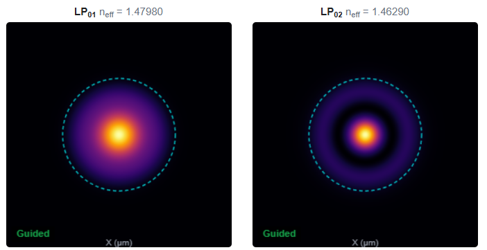
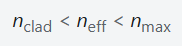
Integer l is the azimuthal mode order; for each l, successive radial solutions are indexed m = 1, 2, …, giving the LP_lm mode set of Gloge's notation [1]. A solution is guided when its effective index n_eff = β/k₀ lies strictly between the cladding and the maximum core index:

Straight-fiber solver: finite differences

The user's (r, n) points are linearly interpolated onto a uniform radial grid of N = 600 points spanning r = 0 to 3×(core radius), with the cladding index applied beyond the core. The above equation is discretized with the standard central-difference stencil, turning it into a tridiagonal generalized eigenvalue problem at each grid index i:

At r = 0 an axisymmetric l'Hôpital limit is applied for the fundamental (l = 0) family; higher azimuthal orders are forced to R(0) = 0, since R(r) ∼ rl near the axis. A Dirichlet condition R(r_max) = 0 truncates the outer boundary. The resulting sparse tridiagonal matrix is diagonalized with a shift-invert Arnoldi method (ARPACK), targeting eigenvalues near σ = (k₀n_max)² and retaining only those inside the guided band of Section 2. The azimuthal order l is swept upward (0, 1, 2, …) until an order yields no further guided solutions, giving the complete LP_lm mode set together with each mode's radial intensity |R(r)|². This finite-difference eigenmode approach follows the general scheme described in [4][5].

Bent-fiber solver: conformal-mapping equivalent index

A fiber bent to radius R_b is treated as an equivalent straight fiber with a spatially tilted index, following the conformal transformation of Heiblum & Harris [6]. The simulator applies the perturbation along the bend-plane axis x:

with R_eff = 1.28 × R_b, the 1.28 correction factor absorbing the photoelastic (stress-optic) contribution beyond pure geometric bending [7]. Equation is then discretized over a square Cartesian grid (90×90 points, half-width 3.5×core radius) with a 5-point Laplacian stencil, and an imaginary quadratic complex absorbing potential (CAP) Γ(x,y) is added in the outer 20% margin to emulate an open radiating boundary:

The absorbing term makes β complex. Its real part gives the usual effective index, n_eff = Re(β)/k₀, while its imaginary part encodes the radiated bend loss:

the 10⁶ factor converting β from µm⁻¹ to m⁻¹. Six leading eigenmodes are extracted per call via shift-invert ARPACK around σ = (k₀ _max n_bent)², each flagged guided when Re(β)² exceeds (k₀n_clad)².

Limitations

The scalar reduction of is only accurate for weakly-guiding, low-birefringence fibers; it does not resolve true vector or polarization-dependent effects. The index profile carries no material dispersion — a single n(r) is supplied per wavelength rather than derived from a Sellmeier model. Accuracy is bounded by grid resolution (N = 600 radially, 90×90 for bent fibers), and the 1.28 stress-optic correction in Equation (4) is a fixed empirical constant rather than a per-geometry calculation.

Read this article to learn how to use the Optoel Simulator:

https://optoelsoft.com/blog/how-to-use-optoel-simulator

References

1. D. Gloge, “Weakly Guiding Fibers,” Applied Optics 10(10), 2252–2258 (1971). doi:10.1364/AO.10.002252

2. A. W. Snyder and J. Love, Optical Waveguide Theory, Chapman & Hall — Ch. 13 (weak-guidance approximation), Ch. 14 (circular fibers).

3. K. Okamoto, Fundamentals of Optical Waveguides, 3rd ed., Elsevier (2021), ISBN 978-0-12-815601-8 — Chs. 2–3.

4. Photonic Devices Research Group, University of Illinois, “Finite Difference Method for Modesolving.”

5. “Yee-mesh-based finite difference eigenmode solver with PML absorbing boundary conditions for optical waveguides and photonic crystal fibers,” Optics Express 12(25), 6165 (2004).

6. M. Heiblum and J. Harris, “Analysis of curved optical waveguides by conformal transformation,” IEEE J. Quantum Electron. 11(2), 75–83 (1975).